Chapter 2 Count distributions: properties and regression models

In this chapter, we present the probability mass function and discuss the main properties of the Poisson, Gamma-Count, Poisson-Tweedie and COM-Poisson distributions.

2.1 Poisson distribution

The Poisson distribution is a notorious discrete distribution. It has a dual interpretation as a natural exponential family and as an exponential dispersion model. The Poisson distribution denoted by \(P(\mu)\) has probability mass function

\[\begin{eqnarray} p(y;\mu) &=& \frac{\mu^y}{y!}\exp\{-\mu\} \nonumber \\ &=& \frac{1}{y!} \exp \{\phi y - \exp\{\phi\} \}, \quad y \in \mathbb{N}_{0}, \tag{2.1} \end{eqnarray}\]

where \(\phi = \log \{\mu\} \in \mathbb{R}\). Hence the Poisson is a natural exponential family with cumulant generator \(\kappa(\phi) = \exp\{\phi\}\). We have \(\mathrm{E}(Y) = \kappa^{\prime}(\phi) = \exp\{\phi\} = \mu\) and \(\mathrm{var}(Y) = \kappa^{\prime \prime}(\phi) = \exp\{\phi\} = \mu\). The probability mass function (2.1) can be evaluated in R through the dpois() function.

In order to specify a regression model based on the Poisson distribution, we consider a cross-section dataset, \((y_i, x_i)\), \(i = 1,\ldots, n\), where \(y_i\)’s are iid realizations of \(Y_i\) according to a Poisson distribution. The Poisson regression models is defined by \[Y_i \sim P(\mu_i), \quad \text{with} \quad \mu_i = g^{-1}(\boldsymbol{x_i}^{\top} \boldsymbol{\beta}).\] In this notation, \(\boldsymbol{x_i}\) and \(\boldsymbol{\beta}\) are (\(p \times 1\)) vectors of known covariates and unknown regression parameters, respectively. Moreover, \(g\) is a standard link function, for which we adopt the logarithm link function, but potentially any other suitable link function could be adopted.

2.2 Gamma-Count distribution

The Poisson distribution as presented in (2.1) follows directly from the natural exponential family and thus fits in the generalized linear models (GLMs) framework. Alternatively, the Poisson distribution can be derived by assuming independent and exponentially distributed times between events (W. M. Zeviani et al. 2014). This derivation allows for a flexible framework to specify more general models to deal with under and overdispersed count data.

As point out by Winkelmann (2003) the distributions of the arrival times determine the distribution of the number of events. Following Winkelmann (1995), let \({\tau_k, k \in \mathbb{N}}\) denote a sequence of waiting times between the \((k-1)\)th and the \(k\)th events. Then, the arrival time of the \(y\)th event is given by \(\nu_y = \sum_{k = 1}^{y} \tau_k\), for \(y = 1, 2, \ldots\). Furthermore, denote \(Y\) the total number of events in the open interval between \(0\) and \(T\). For fixed \(T\), \(Y\) is a count variable. Indeed, from the definitions of \(Y\) and \(\nu_y\) we have that \(Y < y\) iff \(\nu_y \ge T\), which in turn implies \(P(Y < y) = P(\nu_y \ge T) = 1 - F_y(T)\), where \(F_y(T)\) denotes the cumulative distribution function of \(\nu_y\). Furthermore, \[\begin{eqnarray} P(Y = y) &=& P(Y < y+1) - P(Y < y) \nonumber \\ &=& F_y(T) - F_{y+1}(T). \tag{2.2} \end{eqnarray}\]

Equation (2.2) provides the fundamental relation between the distribution of arrival times and the distribution of counts. Moreover, this type of specification allows to derive a rich class of models for count data by choosing a distribution for the arrival times. In this material, we shall explore the Gamma-Count distribution which is obtained by specifying the arrival times distribution as gamma distributed.

Let \(\tau_k\) be identically and independently gamma distributed, with density distribution (dropping the index \(k\)) given by \[\begin{equation} f(\tau; \alpha, \gamma) = \frac{\gamma^{\alpha}}{\Gamma(\alpha)} \tau^{\alpha-1} \exp\{-\gamma \tau\}, \quad \alpha, \gamma \in \mathbb{R}^{+}. \end{equation}\] In this parametrization \(\mathrm{E}(\tau) = \alpha/\gamma\) and \(\mathrm{var}(\tau) = \alpha/\gamma^2\). Thus, by applying the convolution formula for gamma distributions, it is easy to show that the distribution of \(\nu_y\) is given by \[\begin{equation} f_y(\nu; \alpha, \gamma) = \frac{\gamma^{y\alpha}}{\Gamma(y\alpha)} \nu^{y\alpha-1} \exp\{-\gamma \nu\}. \end{equation}\] To derive the new count distribution, we have to evaluate the cumulative distribution function, which after the change of variable \(u = \gamma \alpha\) can be written as \[\begin{equation} F_y(T) = \frac{1}{\Gamma(y\alpha)} \int_0^{\gamma T} u^{n\alpha -1} \exp\{-u\} du, \tag{2.3} \end{equation}\] where the integral is the incomplete gamma function. We denote the right side of (2.3) as \(G(\alpha y, \gamma T)\). Thus, the number of event occurrences during the time interval \((0,T)\) has the two-parameter distribution function \[\begin{equation} P(Y = y) = G(\alpha y, \gamma T) - G(\alpha (y + 1), \gamma T), \tag{2.4} \end{equation}\] for \(y = 0, 1, \ldots\), where \(\alpha, \gamma \in \mathbb{R}^+\). Winkelmann (1995) showed that for integer \(\alpha\) the probability mass function defined in (2.4) is given by \[\begin{equation} P(Y = y) = \exp^{\{-\gamma T\}} \sum_{i = 0}^{\alpha -1} \frac{(\gamma T)^{\alpha y + i}}{\alpha y + i}!. \end{equation}\]

For \(\alpha = 1\), \(f(\tau)\) is the exponential distribution and (2.4) clearly simplifies to the Poisson distribution. The following R function can be used to evaluate the probability mass function of the Gamma-Count distribution.

dgc <- function(y, gamma, alpha, log = FALSE) {
  p <- pgamma(q = 1,
              shape = y * alpha,
              rate = alpha * gamma) -
    pgamma(q = 1,
           shape = (y + 1) * alpha,
           rate = alpha * gamma)
  if(log == TRUE) {p <- log(p)}
  return(p)
}

Although, numerical evaluation of (2.4) can easily be done, the moments (mean and variance) cannot be obtained in closed form. Winkelmann (1995) showed for a random variable \(Y \sim GC(\alpha, \gamma)\), where \(GC(\alpha, \gamma)\) denotes a Gamma-Count distribution with parameters \(\alpha\) and \(\gamma\), \(\mathrm{E}(Y) = \sum_{i = 1}^\infty G(\alpha i, \gamma T)\).

Furthermore, for increasing \(T\) it holds that \[\begin{equation} Y(T) \overset{a}{\sim} N\left(\frac{\gamma T}{\alpha}, \frac{\gamma T}{\alpha^2} \right), \end{equation}\]

thus the limiting variance-mean ratio equals a constant \(1/\alpha\). Consequently, the Gamma-Count distribution displays overdispersion for \(0 < \alpha < 1\) and underdispersion for \(\alpha > 1\). Figure 2.1 presents the probability mass function for some Gamma-Count distributions. We fixed the parameter \(\gamma = 10\) and fit the parameter \(\alpha\) in order to have dispersion index (\(\mathrm{DI} = \mathrm{var}(Y)/\mathrm{E}(Y)\)) equalling to \(0.5\), \(2\), \(5\) and \(20\).

Figure 2.1: Gamma-Count probability mass function by values of the dispersion index (DI).

The Gamma-Count regression model assumes that the period at risk \((T)\) is identical for all observations, thus \(T\) may be set to unity without loss of generality. In the Gamma-count regression model, the parameters depend on a vector of individual covariates \(\boldsymbol{x}_i\). Thus, the Gamma-Count regression model is defined by

\[\begin{equation} \mathrm{E}(\tau_i | \boldsymbol{x}_i) = \frac{\alpha}{\gamma} = g^{-1}(-\boldsymbol{x_i}^\top \boldsymbol{\beta}). \end{equation}\]

Consequently, the regression model is for the waiting times and not directly for the counts. Note that, \(\mathrm{E}(N_i | \boldsymbol{x}_i) = \mathrm{E}(\tau_i | \boldsymbol{x}_i)^{-1}\) iff \(\alpha = 1\). Thus, \(\hat{\boldsymbol{\beta}}\) should be interpreted accordingly. \(-\beta\) measures the percentage change in the expected waiting time caused by a unit increase in \(x_i\). The model parameters can be estimated using the maximum likelihood method as we shall discuss in Chapter 3.

2.3 Poisson-Tweedie distribution

The Poisson-Tweedie distribution (Bonat et al. 2016; Jørgensen and Kokonendji 2015; El-Shaarawi, Zhu, and Joe 2011) consists of include Tweedie distributed random effects on the observation level of Poisson random variables, and thus to take into account unobserved heterogeneity. The Poisson-Tweedie family is given by the following hierarchical specification

\[\begin{eqnarray} Y|Z &\sim& \mathrm{Poisson}(Z) \\ Z &\sim& \mathrm{Tw}_p(\mu, \phi), \nonumber \tag{2.5} \end{eqnarray}\] where \(\mathrm{Tw}_p(\mu, \phi)\) denotes a Tweedie distribution (B. Jørgensen 1987 ; B. Jørgensen 1997) with probability function given by \[\begin{equation} f_{Z}(z; \mu, \phi, p) = a(z,\phi,p) \exp\{(z\psi - k_p(\psi))/\phi\}. \tag{2.6} \end{equation}\]

In this notation, \(\mu = k^{\prime}_p(\psi)\) is the expectation, \(\phi > 0\) is the dispersion parameter, \(\psi\) is the canonical parameter and \(k_p(\psi)\) is the cumulant function. Furthermore, \(\mathrm{var}(Z) = \phi V(\mu)\) where \(V(\mu) = k^{\prime \prime}_p(\psi)\) is the variance function. Tweedie densities are characterized by power variance functions of the form \(V(\mu) = \mu^p\), where \(p \in (-\infty ,0] \cup [1,\infty)\) is an index determining the distribution. The support of the distribution depends on the value of the power parameter. For \(p \geq 2\), \(1 < p < 2\) and \(p = 0\) the support corresponds to the positive, non-negative and real values, respectively. In these cases \(\mu \in \Omega\), where \(\Omega\) is the convex support (i.e. the interior of the closed convex hull of the corresponding distribution support). Finally, for \(p < 0\) the support corresponds to the real values, however the expectation \(\mu\) is positive. Here, we required \(p \geq 1\), to make \(\mathrm{Tw}_p(\mu, \phi)\) non-negative.

The function \(a(z,\phi, p)\) cannot be written in a closed form apart of the special cases corresponding to the Gaussian (\(p = 0\)), Poisson (\(\phi = 1\) and \(p = 1\)), non-central gamma (\(p = 3/2\)), gamma (\(p = 2\)) and inverse Gaussian (\(p = 3\)) distributions (B. Jørgensen 1997). The compound Poisson distribution is obtained when \(1 < p < 2\). This distribution is suitable to deal with non-negative data with probability mass at zero and highly right-skewed (Andersen and Bonat 2016).

The Poisson-Tweedie is an overdispersed factorial dispersion model (Jørgensen and Kokonendji 2015) and its probability mass function for \(p > 1\) is given by \[\begin{equation} f(y;\mu,\phi,p) = \int_0^\infty \frac{z^y \exp{-z}}{y!} a(z,\phi,p) \exp\{(z\psi - k_p(\psi))/\phi\} dz. \tag{2.7} \end{equation}\]

The integral (2.7) has no closed-form apart of the special case corresponding to the negative binomial distribution, obtained when \(p = 2\), i.e. a Poisson gamma mixture. In the case of \(p=1\), the integral (2.7) is replaced by a sum and we have the Neyman Type A distribution. Further special cases include the compound Poisson \((1 < p < 2)\), factorial discrete positive stable \((p > 2)\) and Poisson-inverse Gaussian \((p = 3)\) distributions (Jørgensen and Kokonendji 2015 ; C. C. Kokonendji, Dossou-Gbété, and Demétrio 2004).

In spite of other approaches to compute the probability mass function of the Poisson-Tweedie distribution are available in the literature (Esnaola et al. 2013 ; Barabesi, Becatti, and Marcheselli 2016). In this material, we opted to compute it by numerical evaluation of the integral in (2.7) using the Monte Carlo method as implemented by the following functions.

# Integrand Poisson X Tweedie distributions
integrand <- function(x, y, mu, phi, power) {
    int = dpois(y, lambda = x)*dtweedie(x, mu = mu,
                                        phi = phi, power = power)
    return(int)
}

# Computing the pmf using Monte Carlo
dptw <- function(y, mu, phi, power, control_sample) {
    pts <- control_sample$pts
    norma <- control_sample$norma
    integral <- mean(integrand(pts, y = y, mu = mu, phi = phi,
                               power = power)/norma)
    return(integral)
}
dptw <- Vectorize(dptw, vectorize.args = "y")

When using the Monte Carlo method, we need to specify a proposal distribution, from which samples will be taken to compute the integral as an expectation. In the Poisson-Tweedie case is sensible to use the Tweedie distribution as proposal. Thus, in our function we use the argument control_sample to provide these values. The advantage of this approach is that we need to simulate values once and we can reuse them for all evaluations of the probability mass function, as shown in the following code.

require(tweedie)
set.seed(123)
pts <- rtweedie(n = 1000, mu = 10, phi = 1, power = 2)
norma <- dtweedie(pts, mu = 10, phi = 1, power = 2)
control_sample <- list("pts" = pts, "norma" = norma)
dptw(y = c(0, 5, 10, 15), mu = 10, phi = 1, power = 2,
     control_sample = control_sample)

## [1] 0.0937 0.0590 0.0354 0.0217

dnbinom(x = c(0, 5, 10, 15), mu = 10, size = 1)

## [1] 0.0909 0.0564 0.0350 0.0218

It is also possible to use the Gauss-Laguerre method to approximate the integral in (2.7). In the supplementary material Script2.R, we provide R functions using both Monte Carlo and Gauss-Laguerre methods to approximate the probability mass function of Poisson-Tweedie distribution.

Figure 2.2 presents the empirical probability mass function of some Poisson-Tweedie distributions computed based on a sample of size \(100000\) (gray). Furthermore, we present an approximation (black) for the probability mass function obtained by Monte Carlo integration. We considered different values of the Tweedie power parameter \(p = 1.1\), \(2\), and \(3\) combined with different values of the dispersion index. In all scenarios the expectation \(\mu\) was fixed at \(10\).

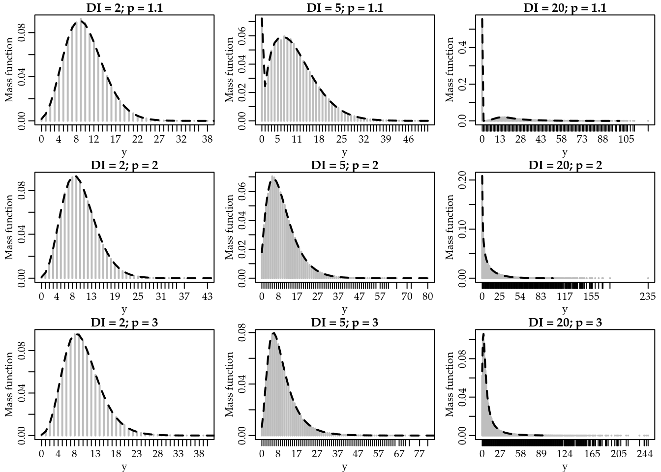
Figure 2.2: Empirical (gray) and approximated (black) Poisson-Tweedie probability mass function by values of the dispersion index (DI) and Tweedie power parameter.

For all scenarios considered the Monte Carlo method provides a quite accurate approximation to the empirical probability mass function. For these examples, we used \(5000\) random samples from the proposal distribution.

Finally, the Poisson-Tweedie regression model is defined by \[Y_i \sim PTw_{p}(\mu_i, \phi), \quad \text{with} \quad \mu_i = g^{-1}(\boldsymbol{x_i}^{\top} \boldsymbol{\beta}),\] where \(\boldsymbol{x}_i\) and \(\boldsymbol{\beta}\) are \((p \times 1)\) vectors of known covariates and unknown regression parameters. The estimation and inference of Poisson-Tweedie regression models based on the maximum likelihood method are challenged by the presence of an intractable integral in the probability mass function and non-trivial restrictions on the power parameter space. In Chapter 3, we discuss maximum likelihood estimation for Poisson-Tweedie regression. Furthermore, in Chapter 4 we extended the Poisson-Tweedie model by using an estimating function approach in the style of Wedderburn (1974).

2.4 COM-Poisson distribution

The COM-Poisson distribution belongs to the family of weighted Poisson distributions. A random variable \(Y\) is a weighted Poisson distribution if its probability mass function can be written in the form \[ f(y; \lambda, \nu) = \frac{\exp^{\{-\lambda\}} \lambda^y w_y}{W y!}, \quad y = 0, 1, \ldots, \] where \(W = \sum_{i = 0}^{\infty} \exp^{\{-\lambda\}} \lambda^i w_i / i!\) is a normalizing constant (Kimberly F. Sellers, Borle, and Shmueli 2012). The COM-Poisson is obtained when \(w_{y} = (y!)^{1-\nu}\) for \(\nu \geq 0\). The series \(W\) for COM-Poisson distribution is denoted by \(Z(\lambda, \nu)\) and can be written as \(\sum_{i=0}^{\infty}\lambda^i/(i!)^\nu\). Note that the series is theoretically divergent only when \(\nu = 0\) and \(\lambda \geq 1\), but numerically for small values of \(\nu\) combined with large values of \(\lambda\), the sum is so huge it causes overflow. The Table 2.1 shows the sums calculated with \(1000\) increments, in other words, \(\sum_{i=0}^{1000}\lambda^i/(i!)^\nu\) for different values of \(\nu\) (horizontal lines) and \(\lambda\) (vertical lines).

Table 2.1: Values for \(Z(\lambda, \nu)\) constant (calculated numerically) to combined values of \(\lambda\) (0.5 to 50) and \(\phi\) (0 to 1)

	0.5	1	5	10	30	50
0	2.00	Inf	Inf	Inf	Inf	Inf
0.1	1.92	7.64	Inf	Inf	Inf	Inf
0.2	1.86	5.25	3.17e+273	Inf	Inf	Inf
0.3	1.81	4.32	1.60e+29	2.54e+282	Inf	Inf
0.4	1.77	3.80	4.71e+10	1.33e+56	Inf	Inf
0.5	1.74	3.47	1.34e+06	3.67e+22	3.32e+196	Inf
0.6	1.72	3.23	2.05e+04	4.99e+12	1.73e+76	4.63e+177
0.7	1.70	3.06	2.37e+03	3.69e+08	4.93e+39	6.93e+81
0.8	1.68	2.92	6.49e+02	2.70e+06	5.09e+24	3.43e+46
0.9	1.66	2.81	2.74e+02	1.47e+05	1.80e+17	2.19e+30
1	1.65	2.72	1.48e+02	2.20e+04	1.07e+13	5.18e+21

In general, the expectation and variance of the COM-Poisson distribution cannot be expressed in closed-form. However, they can be approximated by \[\mathrm{E}(Y) \approx \lambda^{1/\nu} - \frac{\nu - 1}{2 \nu} \quad \text{and} \quad \mathrm{var}(Y) \approx \frac{1}{\nu} \lambda^{1 /\nu}. \] These approximations are accurate when \(\nu \leq 1\) or \(\lambda > 10^{\nu}\). The infinite sum involved in computing the probability mass function of the COM-Poisson distribution can be approximated to any level of precision. It can be evaluated in R using the function dcom() from the compoisson package (Dunn 2012). Figure 2.3 presents some COM-Poisson probability mass functions. We tried to find parameters \(\lambda\) and \(\nu\) in order to have \(\mathrm{E}(Y) = 10\) and dispersion index equals to \(\mathrm{DI} = 0.5, 2, 5\) and \(20\). However, we could not find any parameter combination to have \(\mathrm{DI} = 20\). Probably, it was due to overflow of the sum since \(\nu\) is inversely proportional to the dispersion index (see table 2.1).

Figure 2.3: COM-Poisson probability mass function by values of the dispersion index (DI).

K. F. Sellers and Shmueli (2010) proposed a regression model based on the COM-Poisson distribution where the parameter \(\lambda\) is described by the values of known covariates in a generalized linear models style. The COM-Poisson regression model is defined by \[Y_i \sim CP(\lambda_i, \nu), \quad \text{with} \quad \lambda_i = g^{-1}(\boldsymbol{x_i}^{\top} \boldsymbol{\beta}).\] In this notation, the parameter \(\nu\) is considered the dispersion parameter such that \(\nu > 1\) represents underdispersion and \(\nu < 1\) overdispersion. The Poisson model is obtained for \(\nu = 1\) and as usual we adopt the logarithm link function for \(g\).

2.5 Comparing count distributions

Let \(Y\) be a count random variable and \(\mathrm{E}(Y) = \mu\) and \(\mathrm{var}(Y)\) denote its mean and variance, respectively. To explore and compare the flexibility of the models aforementioned, we introduce the dispersion \((\mathrm{DI})\), zero-inflation \((\mathrm{ZI})\) and heavy-tail \((\mathrm{HT})\) indexes, which are respectively given by \[\begin{equation} \mathrm{DI} = \frac{\mathrm{var}(Y)}{\mathrm{E}(Y)}, \quad \mathrm{ZI} = 1 + \frac{\log \mathrm{P}(Y = 0)}{\mathrm{E}(Y)} \end{equation}\] and \[\begin{equation} \mathrm{HT} = \frac{\mathrm{P}(Y=y+1)}{\mathrm{P}(Y=y)}\quad \text{for} \quad y \to \infty. \end{equation}\]

These indexes are defined in relation to the Poisson distribution. Thus, the dispersion index indicates underdispersion for \(\mathrm{DI} < 1\), equidispersion for \(\mathrm{DI} = 1\) and overdispersion for \(\mathrm{DI} > 1\). Similarly, the zero-inflation index is easily interpreted, since \(\mathrm{ZI} < 0\) indicates zero-deflation, \(\mathrm{ZI} = 0\) corresponds to no excess of zeroes and \(\mathrm{ZI} > 0\) indicates zero-inflation. Finally, \(\mathrm{HT} \to 1\) when \(y \to \infty\) indicates a heavy tail distribution.

For the Poisson distribution the dispersion index equals \(1\) \(\forall \mu\). In the Poisson case, it is easy to show that \(\mathrm{ZI} = 0\) and \(\mathrm{HT} \to 0\) when \(y \to \infty\). Thus, it is quite clear that the Poisson model can deal only with equidispersed data and has no flexibility to deal with zero-inflation and/or heavy tail count data. In fact, the presented indexes were proposed in relation to the Poisson distribution in order to highlight its limitations.

Figure 2.4 presents the relationship between mean and variance, the dispersion and zero-inflation indexes as a function of the expected values \(\mu\) for different scenarios and count distributions. Scenario \(1\) corresponds to the case of underdispersion. Thus, we fixed the dispersion index at \(\mathrm{DI} = 0.5\) when the mean equalling \(10\). Since the Poisson-Tweedie cannot deal with underdispersion, in this scenario we present only the Gamma-Count and COM-Poisson distributions. Similarly, scenarios \(2--4\) are obtained by fixing the dispersion index at \(\mathrm{DI} = 2, 5\) and \(10\) when mean equalling \(10\). In the scenario \(4\) we could not find a parameter configuration in order to have a COM-Poisson distribution with dispersion index equals \(20\). Consequently, we present results only for the Gamma-Count and Poisson-Tweedie distributions. Furthermore, Figure 2.5 presents the heavy tail index for some extreme values of the random variable \(Y\).

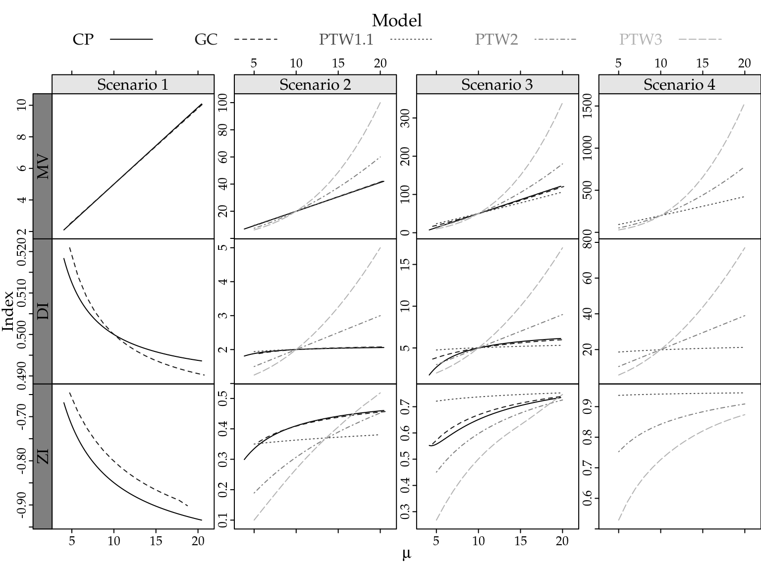
Figure 2.4: Mean and variance relationship (first line), dispersion (DI) and zero-inflation (ZI) indexes as a function of the expected values by simulation scenarios and count distributions.

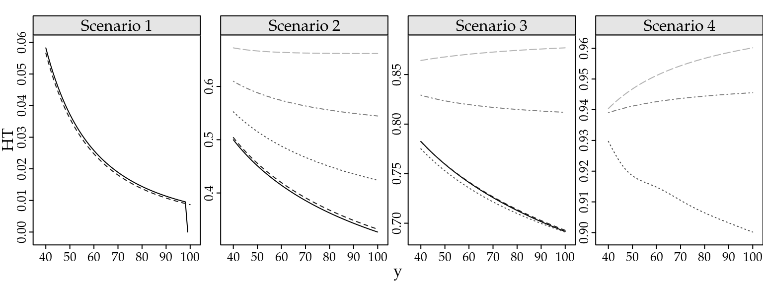
Figure 2.5: Heavy tail index for some extreme values of the random variable Y by simulation scenarios and count distributions.

The indexes presented in Figures 2.4 and 2.5 show that for all considered scenarios the Gamma-Count and COM-Poisson distributions are quite similar. In general, for these distributions, the indexes slightly depend on the expected values and tend to stabilize for large values of \(\mu\). Consequently, the mean and variance relationship is proportional to the dispersion parameter value. In the overdispersion case, the Gamma-Count and COM-Poisson distributions can handle with a limited amount of zero-inflation and are in general light tailed distributions, i.e. \(\mathrm{HT} \to 0\) for \(y \to \infty\).

Regarding the Poisson-Tweedie distributions the indexes show that for small values of the power parameter the Poisson-Tweedie distribution is suitable to deal with zero-inflated count data. In that case, the \(\mathrm{DI}\) and \(\mathrm{ZI}\) are almost not dependent on the values of the mean. Furthermore, the \(\mathrm{HT}\) decreases as the mean increases. On the other hand, for large values of the power parameter the \(\mathrm{HT}\) increases with increasing mean, showing that the model is specially suitable to deal with heavy-tailed count data. In this case, the \(\mathrm{DI}\) and \(\mathrm{ZI}\) increase quickly as the mean increases giving an extremely overdispersed model for large values of the mean. In general, the \(\mathrm{DI}\) and \(\mathrm{ZI}\) are larger than one and zero, respectively, which, of course, show that the corresponding Poisson-Tweedie distributions cannot deal with underdispersed and zero-deflated count data.

For multi-parameter probability function, a desirable feature is the orthogonality betweens parameters. This property leds a series of statistical implications as allows make inference for one parameter without worrying about the values of the other and computationally numerical methods for adjusting distributions with orthogonal parameters are more stable and fast.

The orthogonality is defined by second derivatives of the log-likelihood function, however for the Gamma-Count, Poisson-Tweedie and COM-Poisson and we cannot obtain such derivatives analytically. So we designed a simulation study to evaluate the properties about log-likelihood function for Gamma-Count and COM-Poisson. We used sample size \(n=5000\) for simulate values of Gamma-Count and COM-Poisson following dispersion indexes \(DI=0.5\), \(2\), \(5\) and \(20\) and plot the deviance contours around the maximum likelihood estimation. The Script6.R, in supplement material contains the codes for simulation study. The results are shows in Figure @(fig:ortho).

This graphics presented in Figure 2.6 show that deviance contours are similar a quadratic function (blue dashed contours) for \(DI=0.5\), \(2\), \(5\) in both distributions. However, for the Gamma-Count with \(DI=20\) the quadratic aproximation not as good. For \(DI=20\) and \(\mathrm{E}[Y]=10\) we could not find any parameter combination for COM-Poisson and for Gamma-Count the estimation is innacurate. With respect to orthogonality the Gamma-Count distribution is preferable, the deviance contours are well-behaved, while for COM-Poisson the contour are strongly flat in one direction making the estimation process difficult..

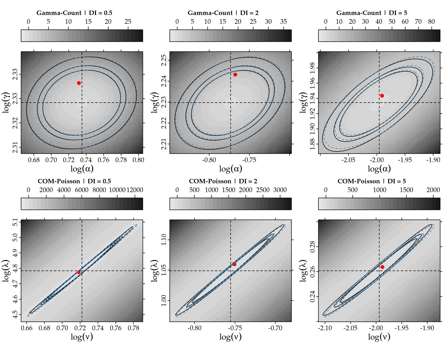
Figure 2.6: Deviance surfaces and quadratic approximation with confidence regions (90, 95 and, 99%) for the two parameters following dispersion indexes (DI) in the simulation study. Dashed lines represents the MLE estimation and red points the parameters used in simulation.

In terms of regression models, the Poisson and Poisson-Tweedie models are easy and convenient to interpret because the expected value is directly modelled as a function of known covariates in a generalized linear models manner. On the other hand, the Gamma-Count specifies the regression model for the expectation of the times between events and, thus requires careful interpretation. The COM-Poisson regression model is hard to interpret and compare with the traditional Poisson regression model, since it specifies the regression model for the parameter \(\lambda\) that has no easy interpretation in relation to the expectation of the count response variable.

Finally, in terms of computational implementation the simplicity of the Poisson regression model is unquestionable. The probability mass function of the Gamma-Count distribution requires the evaluation of the difference between two cumulative gamma distributions. For large values of the random variable \(Y\), such a difference can be time consuming and inaccurately computed. Similarly, the COM-Poisson probability mass function involves the evaluation of a infinity sum, which can be computational expensive and inaccurate for large values of \(Y\). Furthermore, for extreme values of \(\lambda\) combined with small values of \(\nu\) the infinite sum can numerically diverges making impossible to evaluate the probability mass function. Finally, the Poisson-Tweedie probability mass function involves an intractable integral, which makes the estimation and inference based on likelihood methods computationally intensive.